How To: Extended Kalman Filter Using uKal¶

Intro¶

This is a brief introduction on stochastic filtering using an Extended Kalman Filter. A basic model of a vehicle will be discussed and used as the model of exploration for understanding the Kalman Filter. This tutorial covers modeling a systems dynamics, sensing dynamics, setting up all of the required Kalman Filter terms, and running through an example of using such a filter using the uKal library. This tutorial should not serve as a complete course on a Kalman Filter, as it only scrapes the surface of getting to a working filter state.

This tutorial assumes that you have at least basic knowledge of systems (state space, a basic idea of what control theory is, linear system dynamics), classical mechanics from Physics (what position and velocity are, and how they are related), multi-variable calculus (taking a partial derivative, what a Jacobian is, what a vector or matrix function is), basic knowledge of trigonometry (sines and cosines), basic knowledge of statistics (namely: expected value, variances, standard deviations, covariances, and what a random variable is). You must also have a good understanding of the C programming language, and ideally C on an embedded system.

Extended Kalman Filter (EKF) Example¶

First we will discuss modeling a system, modeling how we sense a system, calculating the required Kalman filter terms, and finally setting up your filter using uKal. If you already know what a Kalman filter is, and you already know your required terms, skip to the section on setting up the uKal project (uKal EKF Setup).

The Model¶

Knowing your system model is crucial to using a Kalman filter. In fact, if you ever hear of a situation where a Kalman filter is used but a model is not known, you should be very weary of the filter being used, and perhaps even the principle engineer. The essence of the Kalman filter is to tease out the noise in a known model. If a model is not known, or your model is not "good enough", a Kalman filter may not be right for you.

On the other hand, with some tuning and a good enough model, a Kalman filter can be the best thing that happened to your system if one is not already in use. uKal allows you to start filtering your system for hidden and noisy state estimation and sensor fusion on very low powered machines. This makes even the dumbest microcontroller a potential power house of your system state.

Suppose you have an autonomous vehicle with a microcontroller and some sensors on board. Let's assume that you would like to estimate the following states: the $x$ and $y$ positions of the vehicle on a plane, the velocity, $v$, of the vehicle, and the turn or heading angle, $\theta$, of the vehicle. You may want to do this for the purposes of tracking or controlling one or more of the states in the system; perhaps to implement a navigation algorithm, or to generate a map of the path taken. Assume that you have sensors on board that allow you to only get the position states ($x$ and $y$), but not the angle or velocity states. Furthermore, although your position sensor gives you decent values, they might more error than you can allow, and they might not update fast enough. Say you need to reduce your margin of error from $\pm 2 m$ (common margin for GPS) to $\pm 20 cm$, and you absolutely need new sensor values at a $20 \text{Hz}$ rate ($4$ times faster than most GPS units can update you at) in order meet your system specification.

ekf_tutorial_vehicle

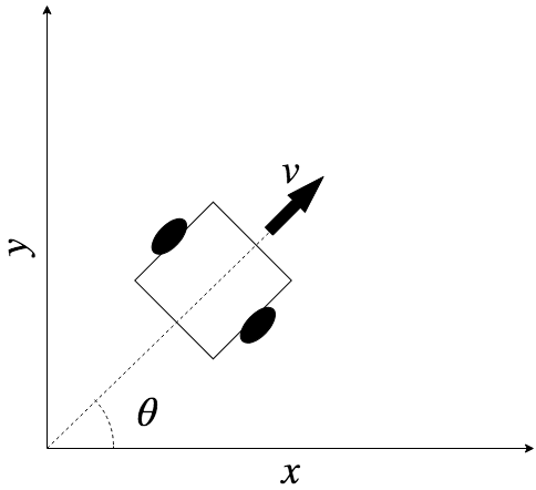
You have modeled the vehicle as a simple point mass moving in 2D space, and you found the ideal state propagation of the system using some classical physics and trigonometry. You calculated that:

$$\dot{x} = v(t)\cos\theta(t)$$$$\dot{y} = v(t)\sin\theta(t)$$

In other words, you figured that the change in your $x$ position is equal to the length traveled in that direction for a single time step plus its previous value. The same can be said for the change in the $y$ state per some unit of time.

Problems With The Model¶

The model is idealistic to say the least for two main reasons:

Problem 1. It is a continuous model of the system. Using any digital computer (e.g. the microcontroller on board the vehicle), we would never be able to propagate such a model because a computer can never yield the limit of time approaching zero (digital quantization, non-ideal oscillators, etc.). Refer to the article: Digital Quantization) for more on why.

Problem 2. The model does not account for all of the intricacies and errors that the real world adds to the system. For example, the slippage in the wheels of the vehicle, the coefficient of static friction on the ground, wind speeds, unbalanced wheels, earthquakes, etc.

Solution 1. Computers can not deal with continuous differential equations such as the models described, but they can deal with discrete difference equations. You can think of these as a rougher approximation of a continuous differential equation with a new associated time step term which basically tells us the time in between points evaluated in the equations. We will refer to this time step as $\Delta T$, and the $k^{th}$, iteration of the equation will be equivalent to $k \Delta T$ units of time since $t = 0$. As long as our model propagates "fast enough" (i.e. $\Delta T$ is small) we should be safely approximating the continuous version of the equations.

Our model as a discrete difference equation as a function of $k$ and $\Delta T$ will now be:

$$x_{k+1} = x_k + v_k \Delta T \cos\theta_k $$$$y_{k+1} = y_k + v_k \Delta T \sin\theta_k $$

Solution 2. If the problems associated with the real world are not drastically going to affect the model, we can simply attribute the errors in our model to a stochastic term added to the end of the state equations. If for some reason these errors in the system are a big enough issue, the extra terms associated with the errors should be modeled into the state equations. We will assume that the extra errors, or "noise", in our "process", or state equations, can be simply attributed to some non-deterministic term summed with our good enough model. We will refer to this non-deterministic noise as $w$. The noise added to the system will always be zero-mean and normal (Gaussian). This way, we can always add some "gain" to the noise down the road to "tune" the noisiness of our model.

With the non-deterministic noise added to our process, our new state equations as stochastic difference equations are:

$$x_{k+1} = v_k \Delta T \cos\theta_k + w_{x_k}$$$$y_{k+1} = v_k \Delta T \sin\theta_k + w_{y_k}$$$$v_{k+1} = v_k + \xi_{v_k} w_{v_k}$$$$\theta_{k+1} = \theta_k +\xi_{\theta_k} w_{\theta_k}$$

where $\xi_v$ and $\xi_\theta$ (described in the section on Covariance and Variances) are the noise gain terms that we can tune that define the stochasticity of the velocity and angle state propagations.

We will set the noise on the $x$ and $y$ state equations to zero, because our only source of error for those terms will be derived from the velocity and angle states. Our final state equations will be:

$$x_{k+1} = v_k \Delta T \cos\theta_k $$$$y_{k+1} = v_k \Delta T \sin\theta_k $$$$v_{k+1} = v_k + \xi_{v_k} w_{v_k}$$$$\theta_{k+1} = \theta_k +\xi_{\theta_k} w_{\theta_k}$$

State Space System¶

Recall that a system of equations can be represented in matrix form. If we say that $\vec{x}$ is a column vector containing our states:

$$ \vec{x} = \begin{bmatrix} x \\ y \\ v \\ \theta \end{bmatrix} $$

We can say that our state vector at the next $\Delta T$ time step $k+1$, $\vec{x}_{k+1}$, is equal to the $k^{th}$ vector function, $\vec{f}_k(\vec{x}_k, \vec{w}_k)$, which maps our last ($k^{th}$) state vector and the process noise into the next ($(k+1)^{th}$) predicted state vector.

$$ \vec{x}_{k+1} = \begin{bmatrix} x_{k+1} \\ y_{k+1} \\ v_{k+1} \\ \theta_{k+1} \end{bmatrix} = \vec{f}_k(\vec{x}_k, \vec{w}_k) = \vec{x}_k + \begin{bmatrix} \Delta T v_k \cos \theta_k \\ \Delta T v_k \sin \theta_k \\ 0 \\ 0 \end{bmatrix} + \begin{bmatrix} 0 \\ 0 \\ \xi_v w_{v_k} \\ \xi_{\theta} w_{\theta_k} \end{bmatrix} $$

Kalman Filtering a Nonlinear System (Enter the EKF)¶

One last thing to note about this model is that it is not linear. The Kalman Filter was originally defined only for linear systems that take on the following state space form:

$$ \dot{\vec{x}} = \Phi \vec{x} + \Gamma \vec{w} $$

and in the discrete difference case as:

$$ \vec{x}_{k+1} = \Phi_k \vec{x}_k + \Gamma_k \vec{w}_k $$

where $\Phi$ maps the previous state vector to the next state vector, $\Gamma$ is the matrix or vector that adds the stochastic terms to state vector. The Kalman Filter equations used to propagate the state estimates require the linear form, and are not defined in our non-linear case explicitly. For an $4$-state state vector, $\vec{x} \in \mathbb{R}^{4}$, $\Phi \in \mathbb{R}^{4 \times 4}$, $\vec{w} \in \mathbb{R}^{2}$, $\Gamma \in \mathbb{R}^{4 \times 2}$.

The $\sin$ and $\cos$ functions are probably the last thing you'd like to see in your model if you hoped to have a linear model. The Extended Kalman Filter (Extended from the linear Kalman Filter) is one of many remedies to this issue of non-linearity. The non-linear state equations will actually be approximated as linear functions in this case via a first order Taylor Approximation, or in other words the first derivative of the state equations. You can think of this simple form of linearizing via approximating the nonlinear function as a tangent line at the point in question on the function for a small period of time (the time step $\Delta T$). uKal also supports the use of the second order filter (SOF), which approximates the function to the second degree. There is a growing group of engineers, and other Kalman filterers, who have an issue with approximating linearity with a Taylor expansion (see The Unscented Kalman Filter), but quite frankly, the EKF is just fine for systems that do not have a high degree of non-linearity. uKal currently does not implement the Unscented Kalman Filter which does not require calculating the Jacobian (first derivative matrix) of the state propagation vector function, $\vec{f}$. The EKF does require the calculation of the Jacobian of $\vec{f}$, so we will do that now. Luckily for most systems, calculating the Jacobian is as simple as typing the state equations into Mathematica or MATLAB, but for a simple system like this, we only need to recall the derivatives of basic terms and function ($\sin$ and $\cos$).

We will let $\Phi_k$ be the $k^{th}$ Jacobian of $\vec{f}_k$. As a side note, for linear systems $\Phi$ is a constant for all iterations, and only needs to be set up once.

$$ \Phi_k = \frac{\partial \vec{f}_k(\vec{x}_k,0)}{\partial \vec{x}_k} = \begin{bmatrix} 1 & 0 & \Delta T \cos \theta_k & -\Delta T v_k \sin \theta_k \\ 0 & 1 & \Delta T \sin\theta_k & \Delta T v_k \cos \theta_k \\ 0 & 0 & 1 & 0 \\ 0 & 0 & 0 & 1 \end{bmatrix} $$

Note that the derivative of the process noise is zero because we only took the partial derivative with respect to the states in the state vector. The EKF requires that we also calculate a separate matrix, $\Gamma$, which contains the partial derivatives of the state equations with respect to the stochastic terms in the $\vec{w}$ vector.

$$ \Gamma_k = \frac{\partial \vec{f}_k(0,\vec{w}_k)}{\partial \vec{w}_k}= \begin{bmatrix} 0 & 0 \\ 0 & 1 \\ 1 & 0\\ 0 & 1 \end{bmatrix} $$

Altogether, our now linearized state equations can be represented in state space matrix form as:

$$ \vec{x}_{k+1} = \Phi_k \vec{x}_k + \Gamma_k \vec{w}_k = \begin{bmatrix} 1 & 0 & \Delta T \cos \theta_k & -\Delta T v_k \sin \theta_k \\ 0 & 1 & \Delta T \sin\theta_k & \Delta T v_k \cos \theta_k \\ 0 & 0 & 1 & 0 \\ 0 & 0 & 0 & 1 \end{bmatrix} \vec{x}_k + \begin{bmatrix} 0 & 0 \\ 0 & 1 \\ 1 & 0\\ 0 & 1 \end{bmatrix} \vec{w}_k $$

The Sensor¶

For a Kalman filter to work, we must also define how we make observations of the system, or in other words: how our sensors measure our states.

As described previously, we know that our sensors measure our Cartesian positions on a plane, but with some noise. Although we are missing sensors for the velocity and angle states, the Kalman filter can do a very good job at estimating those "hidden states". Furthermore, if we had multiple sensors measuring the position states of the system at hand, we could actually fuse the two sensors together in order to achieve a higher degree of state estimate accuracy. This is called "sensor fusion".

The Kalman Filter's observation model dynamics must take on the following linear form:

$$ \vec{z} = H\vec{x} + \vec{\nu} $$

where $\vec{z}$ is our observation vector. $\vec{z}$ is a column vector that contains our sensor readings for the $x$ and $y$ position observations.

$$ \vec{z} = \begin{bmatrix} z_x \\ z_y \end{bmatrix} $$

where our $x$ and $y$ sensor measurements are $z_x$ and $z_y$ respectively.

We know from reading the data sheet of the sensors that there is some noise, $\vec{\nu}$, associated with the sensor measurements.

$$z_x = x + \nu_x$$$$z_y + y + \nu_y$$

Because our model is non-linear, observation dynamics model must be written as follows:

$\vec{z}_k = h_k(\vec{x}_k) + \vec{\nu}$

where $\vec{h}$ is a (potentially nonlinear) vector function that maps our state vector to sensor reading states.

For our two position sensor system, we know that $h_k(\vec{x}_k) = \begin{bmatrix} x_k \\ y_k \end{bmatrix}$, i.e. a vector representing our measured states. The EKF requires that we take partial derivatives of $\vec{z}$ with respect to the state vector, and call the Jacobian of $\vec{h}$, $H$.

$$ H = \frac{\partial \vec{h}_k(\vec{x}_k)}{\partial \vec{x}_k} = \begin{bmatrix} 1 & 0 & 0 & 0 \\ 0 & 1 & 0 & 0 \\ \end{bmatrix}$$

Covariances and Variances¶

We have at this point modeled our state propagation equations, our sensor observation dynamics, and we have even linearized them for use in an EKF. The last thing to do before implementing an Extended Kalman Filter is to define our state and sensor covariance matrices. The whole point of using a stochastic filter like the Kalman Filter is to suppress the variances of our estimated states in a system. We must define some initial values for these variances and covariances before we can begin estimating.

In case you have forgotten the meaning of covariance and variance, in the case of the Kalman Filter, you may think of a covariance as the disjointness in value of two independent states, i.e. "How closely related are the two states in question?". What variance means in this context is simply the disjointness of the state with itself ($\text{cov}(a,a)=\text{var}(a)$), or "How confident am I about the value of this state?".

The State Covariance/Variance Matrix¶

The state covariance matrix, $P$, is a square matrix (with square dimensions equal to the number of states in $\vec{x}$) of covariances (on the off diagonal) and variances (on the diagonal).

Take the equation for $x_{k+1}$ in this example for reference:

$$ x_{k+1} = v_k \Delta T \cos\theta_k $$

Note that $x$ is a function of $v$ and $\theta$. This is to say that our prediction of the value of $x$ in our system is dependent on how well we have predicted the values of $v$ and $\theta$. If our prediction for $\theta$ and/or $v$ is bad, then our prediction of $x$ will therefore be bad. We can also write that $\text{cov}(x,v) > 0$ and $\text{cov}(x, \theta) > 0$, but $\text{cov}(x,y) = 0$ because there appears to be no coupling between those two states. Note that if two states are totally independent of each other, then their covariance is zero.

If our covariance matrix is:

$$ P_k = \begin{bmatrix} \text{var}(x) & \text{cov}(x,y) & \text{cov}(x,v) & \text{cov}(x,\theta) \\ \text{cov}(y,x) & \text{var}(y) & \text{cov}(y,v) & \text{cov}(y,\theta) \\ \text{cov}(v,x) & \text{cov}(v,y) & \text{var}(v) & \text{cov}(v,\theta) \\ \text{cov}(\theta,x) & \text{cov}(\theta,y) & \text{cov}(\theta,v) & \text{var}(\theta) \\ \end{bmatrix} $$

And we know that $\text{cov}(a,b) = \text{cov}(b,a)$, we only have to define the upper or lower triangle of the matrix since it is symmetric across the diagonal.

To generate these values, we can collect some samples from a good enough sensor for the position states for example with the vehicle moving in a known trajectory. We can then find the mean and standard deviation of the sensor data when compared to the known expected values. We then can come up with a good enough initial variance for that position state.

We can just naively state that the velocity state is a function of the two position states (the slope between two position measurements), and simply find the statistical standard deviation of those values, and compound them. The same can be done for the $\theta$ states via the $\arctan$ function of the position states.

It is hard to define a good enough methodology for finding $P$, but as long as the initial guesses for these values are close enough, the Kalman Filter will do an excellent job figuring out the rest. A decent approach to finding $P_0$ is demonstrated in the section on finding the Initial Covariance Matrix.

The Process Noise Covariance/Variance Matrix¶

The process (model) noise covariance matrix, $Q$, must be defined as well. We have two "noisy" states in our state equation ($v$, $\theta$), with a stochastic term gain of $\xi_{v}$ and $\xi_{\theta}$ respectively. The $Q$ matrix with dimensions $2 \times 2$ in this case, will define the variances of the stochastic terms. Recall that multiplying a normal distribution with a variance of $1$ by a positive scalar changes the variance of the distribution to that scalar. A larger scalar multiplier corresponds to more uncertainty in that state. The first row of the $Q$ matrix, for example, in this case will define the variance of the process noise for the velocity state in the first column, and the covariance between the velocity and angle states in the second column.

$$ Q = \begin{bmatrix} \text{var}(v) & \text{cov}(v, \theta) \\ \text{cov}(\theta, v) & \text{var}(\theta) \end{bmatrix} = \begin{bmatrix} \xi_v & 0 \\ 0 & \xi_\theta \end{bmatrix}$$

We previously defined the variance scaling terms in the section on the model. These terms will be derived from our certainty of these states from the estimator. These values often require some tuning. Choose values that you find reduce your variance over time the most. They should be non-zero values on the diagonal, and non-zero on the off diagonal if and only if there is some coupling between the states in the covariance argument.

The Sensor Noise Covariance/Variance Matrix¶

The final matrix that needs to be defined for the filter is the sensor noise covariance matrix, $R$. These values indicate our certainty in our measurements (measurement variances) and how their uncertainties correlate with each other (covariances between state observations). These values are typically found in the datasheet of the sensors used. $R$ tells us how far off our sensor observation dynamics are from our measured states. For example, if we are using a Global Positioning Sensor (GPS) for our position sensing, the datasheet might say that the measurements are within plus or minus $5$ meters. We can then say that the variance of that position state is $5^2$ $\text{meters}^2$.

The covariances in the $R$ matrix define how cross correlated two measured values are. These values are only non-zero if there is some cross coupling between the sensed states. This is a difficult value to find when there is interference between the measured axes for example, and if the values are not in the datasheet, then some tuning may be required.

Initial State Vector & Covariance Matrix¶

Now that you have defined your system's states, how your model affects your states, how you sense your states, and how sure you are about the state equations and sensors, you can finally setup up your Extended Kalman Filter. Luckily for you, if you've made it to this point you are moments away from plugging in your state space terms into a couple of uKal function calls and you're ready to start estimating.

First, let's get everything ready for the filter creation function.

You'll first need an initial guess of your state vector values and your covariance matrix. We will refer to these terms as $\vec{x}_0$ and $P_0$ respectively. Your initial state vector should be your best first guess as to what the values of the states are. You can grab one of the first sensor measurements for the observed states to do this. In the case of the position sensor, we will use our first sensed $x$ position state, $z_{x_0}$, as our initial $x$ guess, $x_0$. We will use $z_{y_0}$ as $y_0$. Recall that velocity, $v_i = \sqrt{v_{x_i}^2 + v_{y_i}^2}$, where $v_{x_i} = \frac{x_i - x_{i-0}}{\Delta T}$. We must therefore use $v_1$ as our initial velocity state because velocity requires two points to calculate. Because of this, we must actually move our initial position guesses to the second sensor measurement to keep our initial state values consistent. The initial angle state $\theta_0$ will be the first heading angle of the vehicle. If this value is known because the vehicle always starts in the same position, then the known value can be used. Otherwise, an $\arctan$ function between the two initial $x$ and $y$ sensor measurements can be used to calculate this value. We will just assume that the initial heading angle state is $\pi$ for simplicity.

Our initial state vector, $\vec{x}_0$ should now look like this:

$$ \vec{x}_0 = \begin{bmatrix} x_1 \\ y_1 \\ v_1 \\ \theta_0 \end{bmatrix} = \begin{bmatrix} z_{x_1} \\ z_{y_1} \\ \sqrt{\Big[{\frac{x_1 - x_0}{\Delta T}}\Big]^2 + {\Big[\frac{y_1 - y_0}{\Delta T}}\Big]^2} \\ \pi \end{bmatrix} $$

Our initial state covariance matrix, $P_0$ will take on the values described in the section on Covariances and Variances, i.e. the confidence in our state vector on the diagonal, and the product of coupled uncertainties on the off diagonal. $P_0$ should explicitly define the variance/covariance matrix for the initial state vector guess. Since our initial guess for $\vec{x}$ can directly from the noisy sensors, we can just find the variance of the noise from the sensors.

For example: We can setup the vehicle at position $(x,y) = (0,0)$ on a plane, and collect $20$ samples of the stationary vehicle. In this case, we might generate the following data from the position sensors:

$$\vec{z}_{1 \dots 20} = \Bigg\{ \vec{z}_1 = \begin{bmatrix} 0.201 \\ 0.191 \end{bmatrix}, \vec{z}_2 = \begin{bmatrix} 0.159 \\ 0.395 \end{bmatrix}, \dots, \vec{z}_{20} = \begin{bmatrix} 0.256 \\ 0.122 \end{bmatrix}\Bigg\}$$

We can then take the standard deviation of the data collected, and refer to those values as the standard deviations of the $x$ and $y$ position sensors ($\sigma_x$ and $\sigma_y$ respectively). Then, $\text{var}(x_0) = \sigma_x^2$ and $\text{var}(y_0) = \sigma_y^2$.

The variance of the velocity state will be the compounded variances from both the $x$ and $y$ states.

If we were to take the variance of this state, we would get:

$$ \text{var}(v_1) = \text{var}\Bigg( \sqrt{\Big[{\frac{x_1 - x_0}{\Delta T}}\Big]^2 + {\Big[\frac{y_1 - y_0}{\Delta T}}\Big]^2} \Bigg) $$

We simply take the variance of each term that has a variance. Recall that the variance of a scalar value, $a$, is its square, $a^2$. Variances can not be negative, e.g. the variance of the term $\text{var}(y_1 - y_0)$ is $\text{var}(y_1) + \text{var}(y_0)$ because $\text{var}(-y_0) = \text{var}(y_0)$ ($\text{var}(-1) = -1^2 = 1$).

$$ \text{var}(v_1) = \sqrt{\Big[{\frac{\text{var}(x_1) + \text{var}(x_0)}{\text{var}(\Delta T)}}\Big]^2 + \Big[{\frac{\text{var}(y_1) + \text{var}(y_0)}{\text{var}(\Delta T)}}\Big]^2} $$

Our initial guess for the first and second $x$ and $y$ states are just as good as each other since the variance suppressing filter has yet to run, i.e. $\text{var}(x_1) = \text{var}(x_0)$ and $\text{var}(y_1) = \text{var}(y_0)$. After combining like terms, we get

$$ \text{var}(v_1) = \sqrt{\Big[{\frac{2\text{var}(x)}{\text{var}(\Delta T)}}\Big]^2 + \Big[{\frac{2\text{var}(y)}{\text{var}(\Delta T)}}\Big]^2} $$

Squaring both terms, and recalling that the variance of the scalar term $\Delta T$ is $\Delta T^2$, we get:

$$ \text{var}(v_1) = \sqrt{{\frac{2^2\text{var}(x)^2}{{\Delta T^2}^2}} + {\frac{2^2\text{var}(y)^2}{{\Delta T^2}^2}}} $$

In our case, where the position states come from the same sensor, and because we are grabbing our initial position state guesses from the same sensor, we will assume that our $x$ and $y$ guess are equally confident, i.e. $\text{var}(x_1) = \text{var}(x_0) = \text{var}(y_1) = \text{var}(y_0)$, yielding:

$$ \text{var}(v_1) = \sqrt{{\frac{2^2\text{var}(x)^2}{\Delta T^4}} + {\frac{2^2\text{var}(x)^2}{\Delta T^4}}} = \sqrt{{2\frac{2^2\text{var}(x)^2}{\Delta T^4}}} = 2\sqrt{2}\frac{\text{var}(x)}{\Delta T^2} $$

We can therefore state that because the initial angle state is a function of the first two values of each of the initial $x$ and $y$ states, $\text{cov}(x_1,\theta_1) = \text{cov}(y_1,\theta_1) = 2\text{var}(x)=2\sigma_x^2$. We can also state that because we know the initial variance of the angle state, we have some associated variance with that known expectation, say $\pi$ (a small constant). Lastly, we found $\text{var}(v_1) = 2\sqrt{2}\frac{\text{var}(x)}{\Delta T^2}$, from this we can state that the covariance between the variance and any one of the position states is $\frac{\sigma_x^2}{\Delta T^2}$.

$$ P_0 = \begin{bmatrix} \text{var}(x_1) & \text{cov}(x_1,y_1) & \text{cov}(x_1,v_1) & \text{cov}(x_1,\theta_1) \\ \text{cov}(y_1,x_1) & \text{var}(y_1) & \text{cov}(y_1,v_1) & \text{cov}(y_1,\theta_1) \\ \text{cov}(v_1,x_1) & \text{cov}(v_1,y_1) & \text{var}(v_1) & \text{cov}(v_1,\theta_1) \\ \text{cov}(\theta_1,x_1) & \text{cov}(\theta_1,y_1) & \text{cov}(\theta_1,v_1) & \text{var}(\theta_1) \\ \end{bmatrix} = \begin{bmatrix} \sigma_x^2 & 0 & \frac{\sigma_x^2}{\Delta T^2} & 2\sigma_x^2 \\ 0 & \sigma_x^2 & \frac{\sigma_x^2}{\Delta T^2} & 2\sigma_x^2 \\ \frac{\sigma_x^2}{\Delta T^2} & \frac{\sigma_x^2}{\Delta T^2} & 2\sqrt{2}\frac{\text{var}(x)}{\Delta T^2} & 0 \\ 2\sigma_x^2 & 2\sigma_x^2 & 0 & \pi \\ \end{bmatrix}$$

Note that the zeros in the matrix indicate that there is no cross coupling of information that interferes with the prediction of the respective initial guesses for those two states.

We now have a good first guess for the $Q$ matrix, but this may still require some tuning. Note that the matrix elements must be with respect to a time step $\Delta T$ because they relate the state equation noise across a time step.

$$ Q \approx \begin{bmatrix} \text{var}(v) & \text{cov}(v, \theta) \\ \text{cov}(\theta, v) & \text{var}(\theta) \end{bmatrix} = \begin{bmatrix} 2\sqrt{2}\frac{\text{var}(x)}{\Delta T^2}\Delta T & 0 \\ 0 & \pi \Delta T \end{bmatrix}$$

And because we now know the variances of the sensor reading, we can fill in the sensor noise covariance matrix, $R$,

$$ R = \begin{bmatrix} \text{var}(z_x) & \text{cov}(z_x, z_y) \\ \text{cov}(z_y, z_x) & \text{var}(z_y) \end{bmatrix} = \begin{bmatrix} \text{var}(x_0) & 0 \\ 0 & \text{var}(y_0) \end{bmatrix} = \begin{bmatrix} \sigma_x^2 & 0 \\ 0 & \sigma_y^2 \end{bmatrix}$$

Note that the covariances are zero in this ideal case, but this is common to have coupled sensor observation noise.

The Kalman Filter Equations¶

The Kalman Filter works to suppress uncertainty (variances) in the predictions and estimates of the state vector. It does this by combining a prediction of the states from the state model equations, and from actual sensor observations of the states (or related states). In order to weigh these terms, a term is introduced, called the Kalman Gain matrix, which is essentially a matrix of weights that weigh various state predictions and observations against each other.

Recall that after linearizing the nonlinear system, we have that:

$$ x_{k+1} = \vec{f}_k(\vec{x}_k, \vec{w}_k) $$$$ \vec{z}_k = \vec{h}_k(\vec{x}_k) + \vec{\nu}_k $$$$ \Phi_k = \frac{\partial \vec{f}_k(\vec{x}_k(-),0)}{\partial \vec{x}_k},\ \Gamma_k = \frac{\partial \vec{f}_k(\vec{x}_k(-),0)}{\partial \vec{w}_k},\ H_k = \frac{\partial \vec{h}_k(\vec{x}_k(-),0)}{\partial \vec{x}_k}$$

Here the parenthetic minus sign, $(-)$, indicates that the term is predicted. The Kalman Filter can function in two major ways: predictions and updates.

Kalman Predictions¶

We predict the state vector and covariance matrix for two reasons. First, we may like to know the current prediction of the state vector in the absence of a sensor update. A prediction is also required for the Kalman Filter to properly calculate its gain matrix for the purposes of a sensor update.

A prediction in the Kalman Filter sense is a simple propagation of the state vector (without any added noise) via the state propagation vector function, $\vec{f}$. We will refer to a predicted state vector at iteration $k$, as:

$$ \vec{x}_{k+1}(-) = \vec{f}_k(\vec{x}_k, 0) $$

We must also calculate the predicted covariance matrix, $P(-)$, of the system after a prediction. This is done via:

$$ P_{k+1}(-) = \Phi_k P_k \Phi_k^T + \Gamma_k Q_k \Gamma_k^T $$

Note that the predicted covariance matrix is only a function of the last covariance matrix and the state equation terms and covariances. This is because the prediction was the result of propagating the model itself, and not with the direct assistance of the sensor(s). Also note that the next covariance matrix is a function of the last covariance matrix. The covariance matrix is in a way the hysteresis term of the Kalman Filter, as it connects the predictions to the updates as we will soon see.

It is safe to assume that the uncertainties (variances) in the state estimates after a prediction increase. This is because information from the reality of the situation (from sensor observations) is further back in time after a prediction. For linear systems (unlike our example) we are actually guaranteed two things from the Kalman Filter: the variance drops after a sensor update, and the state variance increase in the absence of sensor updates. This is why a Kalman Filter is referred to as an Optimal Estimator in the linear case. The filter works to eliminate uncertainties in the state vector. There is no such guarantee in in the nonlinear case. In fact, there is no "optimal" filter for nonlinear systems. Luckily, the EKF does a good enough job, and will likely perform much better than a non-Kalman filtered system in terms of systematically reducing state estimate variances.

To update a Kalman Filter using uKal, make a call to ukal_model_predict().

Kalman Updates¶

We only update the filter when we have actual sensor observations to update our filter with. We can hand the filter raw noisy sensor measurements, and expect to get a newly filtered estimated state vector, along with the variances (uncertainties) of the current state estimates. Note that you must make a prediction of both the state vector and the covariance matrix before updating the filter with a sensor measurement.

First, we calculate the current Kalman Gain matrix, $K$, which is a function of the last predicted covariance matrix, $P_{k+1}(-)$, the linearized sensor observation matrix, $H$, and the sensor noise covariance matrix, $R$. The Kalman Gain matrix is the result of a classic optimization derivation. This derivation will not be done in this tutorial as this document is to serve as a brief introduction to the filter and a manual for the uKal library. If you are interested in learning more about the (beautiful) derivations of the Kalman Gain matrix, amongst other terms, see MIT - Tutorial: The Kalman Filter.

$$ K_{k+1} = P_{k+1}(-)H_{k+1}^T (H_{k+1}P_{k+1}(-)H_{k+1}^T + R_{k+1})^{-1} $$

If we expand the predicted covariance matrix terms inside of the Kalman Gain calculation, we find:

$$ K_{k+1} = (\Phi_k P_k \Phi_k^T + \Gamma_k Q_k \Gamma_k^T)H_{k+1}^T (H_{k+1}(\Phi_k P_k \Phi_k^T + \Gamma_k Q_k \Gamma_k^T)H_{k+1}^T + R_{k+1})^{-1} $$

A bit messy, but it becomes clear that the Kalman Gain matrix is a function of every term in the filter except for the state vector and the sensor measurement vector.

The update step then calculates the new estimate of the state vector as a function of the predicted value of the state vector, the Kalman Gain matrix, the sensor measurements, and the observation vector function.

$$ \vec{x}_{k+1} = \vec{x}_{k+1}(-) + K_{k+1}(\vec{z}_{k+1} - h_{k+1}(\vec{x}_{k+1}(-)) $$

Let's look at some of the terms a little closer. First, we have the following term which compares our actual sensor measurement to our predicted sensor measurement:

$$ \vec{z}_{k+1} - h_{k+1}(\vec{x}_{k+1}(-) $$

this term is referred to as the innovation of the update. It is the residual error of our prediction and our actual observation. We multiply this term by the Kalman Gain matrix, $K_{k+1}$, to weigh our actual observation against our expected. We then add our last predicted value to the innovated term. Note that the estimate of the state vector contains every possible term in the filter when expanded.

Finally, we must update our covariance matrix, $P$, to reflect our new sensor update.

$$ P_{k+1} = (I - K_{k+1}H_{k+1})P_{k+1}(-) $$

Using uKal, you can update your filter's terms by simply calling ukal_update() with the new sensor measurements. This saves you from rolling your own matrix math library which computes matrix inversions, transposes, multiplications, additions, etc.

Using uKal for State Estimation¶

At this point, you know your values for $\vec{x}_0$, $P_0$, $\vec{f}_k(\vec{x}_k,0)$, $\Phi_k$, $\Gamma_k$, $Q$, $h_k(\vec{x}_k)$, $H$, and $R$. You will need to pipe in the ability to grab a sensor measurement, we'll call $\vec{z}$. In this example, we will call the function that does this: get_sensor().

Let us examine a possible work-flow for setting up a uKal EKF. In this example, we will first declare the filter and all of the required terms. Because the terms are all matrices and vectors, we will be using uLAPack (a linear algebra package I designed for this explicit purpose). uLAPack is configured to use statically allocated objects, and is designed to be safe on embedded systems with critical tasks. After declaring the terms, the objects are initialized to their intended dimensions, and their initial values are set. The filter is then initialized with the initialized terms, and the filter can begin to run.

First we want to include ukal.h for the Kalman Filter library function declarations, the filter types, and the filter error code types. We want to also include ulapack.h for the matrix/vector manipulation functions.

// @file some_c_file.c
// uKal EKF Setup Example

#include "ulapack.h" // include the matrix math library for data
#include "ukal.h" // include the Kalman filter library

uKal does not compute the Jacobian of $\vec{f}$ and $\vec{h}$. You must pipe in the ability to compute those values (as done in the following example). The functions simply pass back by value the matrix objects that they set, and then a later call to set the terms within the filter must be made. Recall that we derived these exact Jacobian terms in the tutorial.

// Gets the Jacobian of f(x)
static void get_phi(Matrix_t * const Phi, 
                    const Matrix_t * const x, 
                    const MatrixEntry_t dt) {
    // grab the velocity and angle states from the state vector
    MatrixEntry_t v = x->entry[2][0];
    MatrixEntry_t theta = x->entry[3][0];

    // since there are ones on the diagonal of Phi, just set it to
    // the identity initially.
    ulapack_eye(Phi);

    // fill in the values of Phi_k as calculated via the Jacobian
    ulapack_edit_entry(Phi, 0, 2, dt*cos(theta));
    ulapack_edit_entry(Phi, 1, 2, dt*sin(theta));

    ulapack_edit_entry(Phi, 0, 3, -1*dt*v*sin(theta));
    ulapack_edit_entry(Phi, 1, 3, dt*v*cos(theta));
}

// Gets the state propagation vector, f(x)
static void get_fx(Matrix_t * const fx,
                   const Matrix_t * const x,
                   const MatrixEntry_t dt) {
    // isolate the velocity and angle states
    MatrixEntry_t v = x->entry[2][0];
    MatrixEntry_t theta = x->entry[3][0];

    ulapack_edit_entry(fx, 0, 0, x->entry[0][0] + dt * v * cos(theta));
    ulapack_edit_entry(fx, 1, 0, x->entry[1][0] + dt * v * sin(theta));
    ulapack_edit_entry(fx, 2, 0, x->entry[2][0]);
    ulapack_edit_entry(fx, 3, 0, x->entry[3][0]);
}

// Gets the sensor observation vector, h(x)
static void get_hx(Matrix_t * const hx, 
                   const Matrix_t * const x) {
    ulapack_edit_entry(hx, 0, 0, x->entry[0][0]);
    ulapack_edit_entry(hx, 1, 0, x->entry[1][0]);
}

Your main function may look like the following. Here we declare some familiar variables for the state vector, Kalman Filter terms, and the filter object itself. We also define the number of states in our system ($4$), and the number of sensor observations ($2$), since they may be referenced throughout the program.

Filter_t filter; // the filter object for the vehicle 

const Index_t n_states = 4; // we have four states in our system (x, y, v, theta)
const Index_t n_measurements = 2; // we have two measurement states (x, y)

const MatrixEntry_t dt = 0.33333; // define the time step between model updates \Delta T

// the following standard deviations have been precalculated using std() in MATLAB from
// 20 sensor samples.
const MatrixEntry_t stdx = 1.3940; // our roughly found standard deviation for our x state
const MatrixEntry_t stdy = stdx; // assume that our model for y is as noisy as x

const MatrixEntry_t varx = stdx * stdx; // var(x) = std(x)^2
const MatrixEntry_t vary = varx; // same variance as x because same std of x

const MatrixEntry_t varv = 2*sqrt(2)*(varx / (dt * dt)); // as derived in the example
const MatrixEntry_t vartheta = 3.14; // as explained in the example

/*
 * Set up two measurement vectors with proper dimensions.
 * Store the first and second sensor measurements to calculate 
 * initial velocity.
 */
Matrix_t y1;
Matrix_t y;
ulapack_init(&y, n_measurements, 1);
ulapack_init(&y1, n_measurements, 1);

/*
 * Take two measurements a period of dt apart.
 */
get_sensor_data(&y);
wait(dt); // perhaps some sort of a blocking function
get_sensor_data(&y1);

/*
 * Set up the State vector to be a column vector with the initial values
 * discussed in the example.
 */
Matrix_t x;
ulapack_init(&x, n_states, 1);
ulapack_edit_entry(&x, 0, 0, y1.entry[0][0]); // x0
ulapack_edit_entry(&x, 1, 0, y1.entry[1][0]); // y0
ulapack_edit_entry(&x, 2, 0, sqrt(
                                ((y1.entry[0][0] - y.entry[0][0]) / dt) *
                                ((y1.entry[0][0] - y.entry[0][0]) / dt) + 

                                ((y1.entry[1][0] - y.entry[1][0]) / dt) *
                                ((y1.entry[1][0] - y.entry[1][0]) / dt) 
                              ); // v0 = sqrt(vx1^2 + vy1^2)

ulapack_edit_entry(&x, 3, 0, 3.1416); // theta0 = pi

/*
 * The state propagation matrix; Jacobian of f(x).
 * These values change every iteration of the filter.
 */
Matrix_t Phi;
ulapack_init(&Phi, n_states, n_states);
get_phi(&Phi, &x, dt);

/*
 * The state process noise.
 * The values are constant after this.
 */
Matrix_t gamma;
ulapack_init(&gamma, n_states, 2);
ulapack_set(&gamma, 0.0);
ulapack_edit_entry(&gamma, 2, 0, 1.0);
ulapack_edit_entry(&gamma, 3, 1, 1.0);

/*
 * The state process noise covariance matrix.
 * Constant.
 */
Matrix_t Q;
ulapack_init(&Q, gamma.n_cols, gamma.n_cols);
ulapack_set(&Q, 0.0);
ulapack_edit_entry(&Q, 0, 0, 5*5*dt);
ulapack_edit_entry(&Q, 1, 1, .5*.5*dt);

/*
 * The state covariance matrix.
 */
Matrix_t P;
ulapack_init(&P, n_states, n_states);
ulapack_edit_entry(&P, 0, 0, varx);
ulapack_edit_entry(&P, 1, 1, vary);
ulapack_edit_entry(&P, 2, 2, varv);
ulapack_edit_entry(&P, 3, 3, vartheta);

ulapack_edit_entry(&P, 0, 2, 2*varx / (dt * dt));
ulapack_edit_entry(&P, 2, 0, 2*varx / (dt * dt));
ulapack_edit_entry(&P, 1, 2, 2*varx / (dt * dt));
ulapack_edit_entry(&P, 2, 1, 2*varx / (dt * dt));

ulapack_edit_entry(&P, 0, 3, 2*varx);
ulapack_edit_entry(&P, 3, 0, 2*varx);
ulapack_edit_entry(&P, 1, 3, 2*varx);
ulapack_edit_entry(&P, 3, 1, 2*varx);

/*
 * The observation matrix; Jacobian of h(x).
 * The matrix is constant so we only need to set it once.
 */
Matrix_t H;
ulapack_init(&H, n_measurements, n_states);
ulapack_set(&H, 0.0);
ulapack_edit_entry(&H, 0, 0, 1.0);
ulapack_edit_entry(&H, 1, 1, 1.0);

/*
 * The sensor noise matrix.
 */
Matrix_t R;
ulapack_init(&R, n_measurements, n_measurements);
ulapack_set(&R, 0.0);
ulapack_edit_entry(&R, 0, 0, (stdx*stdx) / 3);
ulapack_edit_entry(&R, 1, 1, (stdy*stdy) / 3);

/*
 * The state vector propagation function, f(x).
 */
Matrix_t fx;
ulapack_init(&fx, n_states, 1);

/*
 * The sensor observation vector, h(x).
 */
Matrix_t hx;
ulapack_init(&hx, n_measurements, 1);
get_hx(&hx, &x);

After initializing all of the term dimensions and values, call ukal_filter_create() to set up your filter object. The function requires a pointer to the filter object itself, the filter type (either linear, ekf, or sof), the number of states and observations, the state model terms, the sensor observation terms, and the covariance matrices.

/*
 * Initialize the filter object with the state space terms.
 */
ukal_filter_create(&filter, ekf,             // set up our filter object as an EKF
                   n_states, n_measurements, // with 4 states, and 2 observations
                   &Phi, &gamma, &x, &Q,     // Set the process terms
                   &P,                       // set the initial cov matrix
                   &H, &R);                  // set the obs and sensor noise matrices

The filter is now ready to run properly. In this loop we predict the state vector at every $\Delta T$ time period (dt). If a sensor measurement occurs, we update the filter with the observation only after previously predicting the state.

// run the filter
for (;;) { // loop until vehicle dies

    // get the predicted state vector by propagating f(x).
    // set the internal filter value to the propagated value.
    get_fx(&fx, &filter.x, dt);
    ukal_set_fx(&filter, &fx);

    // calculate the value of the Jacobian given the current state vector.
    // set the internal value of Phi_k.
    get_phi(&Phi, &filter.x, dt);
    ukal_set_phi(&filter, &Phi));

    // Propagate the internal predicted model of the EKF.
    // This updates the internal state, filter.x, and the predicted
    // covariance matrix, filter.P.
    ukal_model_predict(&filter);

    // check if we got a sensor update.
    if (new_sensor_data()) {
        // get a sensor update
        get_sensor_data(&y);

        // calculate observation matrix Jacobian given the current state.
        // set the internal value filter.H = Hx
        get_hx(&hx, &filter.x);
        ukal_set_hx(&filter, &hx);

        // update the internal filter model given the new update from the sensors.
        // This update the internal model's state vector, Kalman Gain matrix,
        // and covariance matrix.
        ukal_update(&filter, &y);
    }

    /*
     * The current confidence in our state estimates are the diagonals of filter.P
     */

    /*
     * The current state estimates are in filter.x
     */
    // do something with Kalman filtered state estimated: filter.x

    /*
     * Our filter should only operate on the period of dt.
     */
    // wait until the next period
}